Quantum Computer Simulator

Basics: How Does It Work?

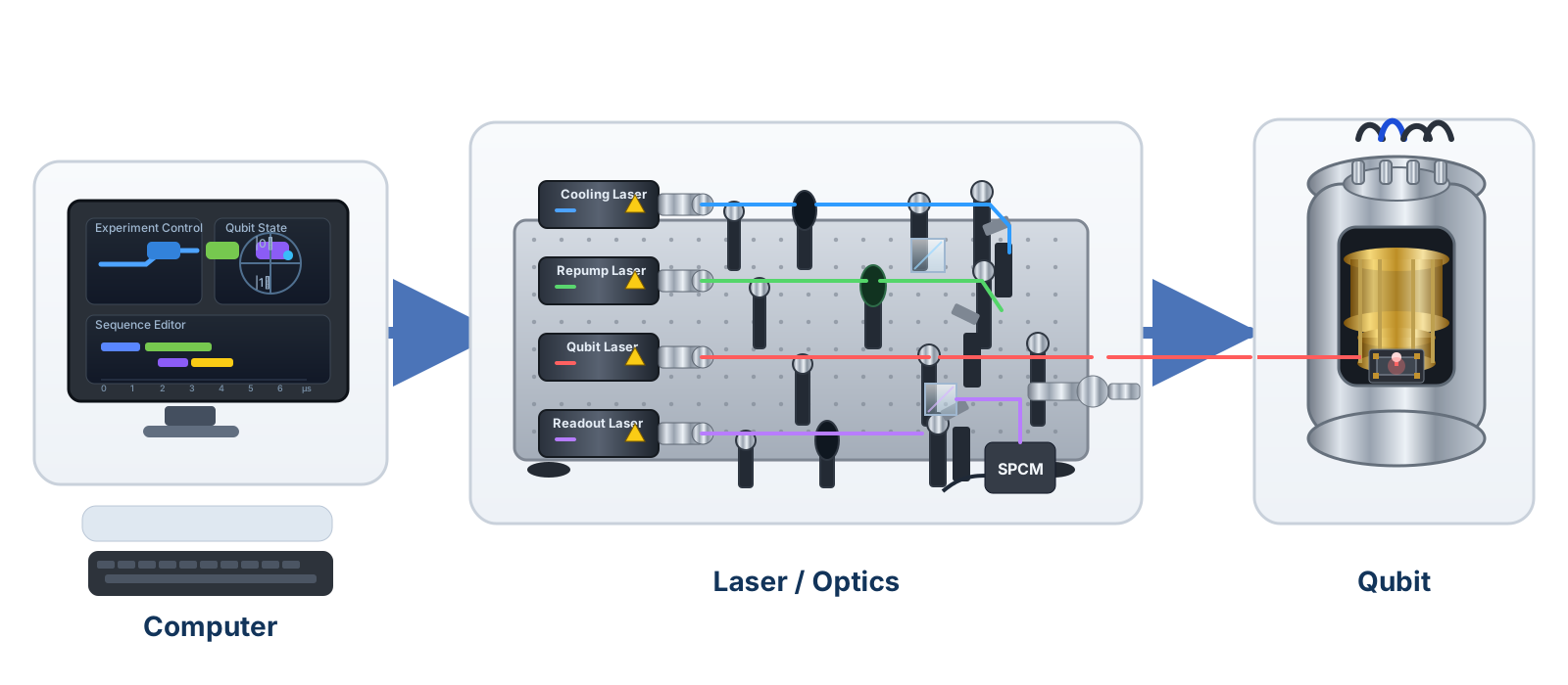
From program to physical qubit

A real quantum computer is more than a chip. Classical control electronics translate the circuit into precise pulses. In the example shown, cooling, repump, qubit, and readout lasers shape these signals on an optical table and direct them into a shielded vacuum chamber. There they change and measure the qubit state; the measurement result then returns to the classical computer.

Qubit & basis states

A classical bit is either 0 or 1. A qubit can additionally exist in a superposition of the two basis states |0⟩ and |1⟩. With several qubits, all basis states are written as a bit string, e.g. |10⟩ for 2 qubits – where q0 in this simulator is always the most significant (left) bit.

Superposition

A qubit in superposition simultaneously carries components of several basis states. These components are described as complex amplitudes; the squared magnitude of an amplitude gives the probability of obtaining the corresponding state in a measurement.

The Bloch sphere

The state of a single qubit can be visualized as an arrow in a sphere: the north pole represents |0⟩, the south pole |1⟩, and all points on the equator are equally weighted superpositions – the phase determines the direction along the equator in which the arrow points. The rotation gates rx, ry, and rz rotate the arrow around the respective axis, phase gates like S and T rotate it around the Z axis. With entangled qubits, the arrow shrinks toward the center of the sphere: the individual qubit then no longer has a pure state of its own – so entanglement becomes literally visible.

Measurement & shots

measureAll() measures all qubits at once and ends the circuit. Since a single measurement only yields one random result, the circuit is conceptually measured "shots" times with run({ shots }), so that the probability distribution shows up as a histogram. The exact probabilities are additionally computed directly from the state vector, independent of the randomness of the shots.

Hadamard gate

The Hadamard gate h(q) takes a qubit from a definite state (|0⟩ or |1⟩) into an equally weighted superposition of |0⟩ and |1⟩ – so about 50% / 50% when measured.

Phase gates: S and T

The gates s(q) and t(q) do not change the measurement probabilities of a single qubit; they only rotate the phase of the |1⟩ amplitude – S by 90°, T by 45°. They only show their effect in combination with superposition: between two Hadamard gates, the phase decides how amplitudes combine or cancel out (interference). The dagger variants sdg(q) and tdg(q) rotate exactly the opposite way and undo S and T. The rule is: two T make an S, two S make a Z.

CNOT & conditional entanglement

The CNOT gate cnot(control, target) flips the target qubit exactly when the control qubit is in state |1⟩. If the control qubit is in superposition beforehand, this can create entanglement – the two qubits can then no longer be described independently of each other, as in the Bell state example. If the control qubit is in a definite basis state instead, CNOT only performs a conditional bit flip without entanglement. So not every CNOT automatically creates entanglement.

CZ: the symmetric relative of CNOT

The CZ gate cz(a, b) inverts the sign of the amplitude exactly when both qubits are |1⟩. Unlike CNOT, there is no control and no target qubit – the gate acts identically on both qubits, which is why it is drawn as two connected dots in the diagram. CZ and CNOT can be converted into each other: a CNOT is a CZ whose target qubit is passed through a Hadamard gate before and after. CZ is a central building block of many algorithms, such as Grover search.

GHZ state: entanglement as a trio

The GHZ state (named after Greenberger, Horne, and Zeilinger) extends the Bell state principle to three qubits: one Hadamard gate plus two CNOTs entangle all three so that measurement only yields |000⟩ or |111⟩ – never mixed bit strings. No qubit has a state of its own anymore; the information lies exclusively in the shared correlation.

Deutsch algorithm: the smallest quantum advantage

The Deutsch algorithm answers, with a single evaluation of an unknown oracle, a question for which a classical computer needs two evaluations: is the function constant or balanced? The trick is to send the input through the oracle in superposition – thanks to interference, the answer afterwards is unambiguously encoded in the input qubit. The principle behind it (phase kickback) is at the core of almost all quantum algorithms.

Grover search: amplifying amplitudes

Grover search finds a marked entry in an unsorted set with significantly fewer queries than classically required. An oracle marks the sought state with a phase flip (here via a CZ gate), then the diffusion operator amplifies the marked amplitude at the expense of all others. With 2 qubits, a single iteration is enough to measure the hit with 100% probability.

Reversible addition: from quantum.add() to a circuit

The program code editor above translates quantum.add({ a, b }) into a circuit of X, CNOT, and CCNOT gates (Toffoli) that reproduces classical addition in a purely reversible way: every gate can be undone exactly, because no information is discarded. A CCNOT gate (ccnot(c1, c2, target)) flips the target qubit only when both control qubits are |1⟩ – that is sufficient as a building block to rebuild any classical circuit reversibly, including a full adder with carry. The inputs A and B are first initialized as definite basis states (no superposition) using X gates. Because the entire circuit therefore only passes through definite states instead of superpositions, the measurement at the end yields exactly one result with 100% probability – the classically correct sum. That is why quantum.add() produces a deterministic result despite the quantum simulation, instead of several possible states with probabilities below 100%.

Subtraction: addition in reverse

Because every gate of a quantum circuit is exactly invertible, the complete adder circuit can be executed backwards – and the addition becomes a subtraction: quantum.subtract({ a, b }) uses exactly the gates of the adder in reverse order and thereby computes a − b. This is not a gimmick but the basic principle of reversible computation: no computation step destroys information, every step can be undone. In this version, a ≥ b is required so that no negative result occurs.

Multiplication: quantum.multiply()

Multiplication here emerges from exactly the same reversible building blocks as addition: following the schoolbook method, factor a is added several times in shifted positions – matching the set bits of factor b. Each partial addition is the same reversible ripple-carry adder; the carry flows into the next product bit each time. Because the result register grows with the product, the factors are limited to 3 bits (0–7) here – only then do factor, product and carry qubit together fit into this simulator's 10 qubits.

Division: quantum.divide()

Division also uses only reversible building blocks: quantum.divide({ a, b }) performs long division built from shifted, reversible subtractions of the divisor from the remainder register; the result is the quotient and the remainder (a = quotient · b + remainder). Because dividend, divisor, quotient and a borrow qubit must all fit into the 10 qubits together, division is the most strongly constrained operation: bits(a) + bits(b) + bits(a÷b) + 1 ≤ 10 must hold, and the divisor b must be ≥ 1 (no division by zero). If an input does not fit the budget, the editor reports it instead of computing.

True randomness: quantum.random()

Classical computers cannot generate true randomness – their "random numbers" come from deterministic algorithms (pseudo-randomness). A quantum computer can: quantum.random({ bits }) puts each bit into a 50/50 superposition using a Hadamard gate, and only the measurement decides – fundamentally unpredictably – which value comes out. On real quantum hardware this is physically true randomness; this simulator imitates it with the pseudo-randomness of your browser.

Simulator vs. real quantum hardware

This simulator computes the state exactly using classical floating-point arithmetic in your browser – this only works because exclusively very small circuits with up to 10 qubits are considered here. Real quantum computers use physical qubits, are error-prone (decoherence, noise), and their advantage only shows with much larger circuits that can no longer be simulated classically in practice. This tool is a learning tool, not a real quantum processor.